The go kart was finally complete with suspension and all, but the go kart was disappointment in corners and on straightways. The wheels would bend over in corners and the suspension was too soft bottoming out constantly.
These problems could have been addressed before the go kart was even finished with vector loop equations, or an mechanical analysis of the go kart suspension. The mechanical analysis begins with an understanding of basic math and as we discussed last time, trigonometry.
The purpose of the mechanical analysis is to determine the spring rate required for the spring, and the overall design configuration so that the wheels hit the ground properly for optimum cornering and straightway characteristics.
There are several designs, however, we will start out with a simple suspension component: A-Arm-Strut Layout.
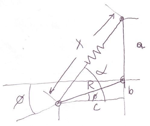
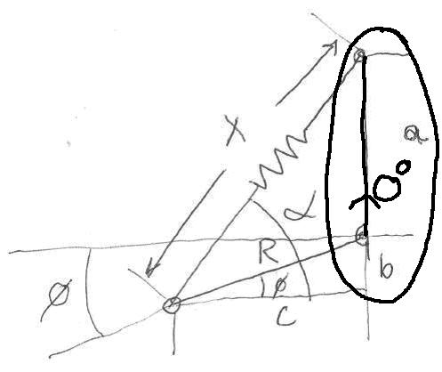
A-Arm-Strut Suspension Layout
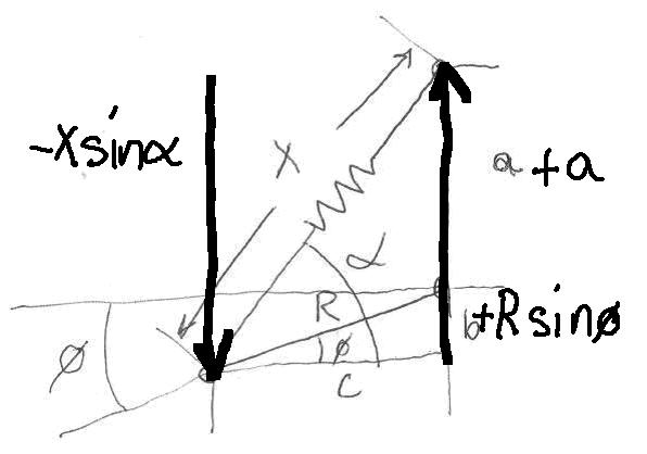
What is shown is basically an obtuse triangle with sides x, R and a. “x” is the spring component which shrinks (or shortens in length) when a bump is hit. The easiest way to evaluate the suspension is to relate everything to the angle THETA.
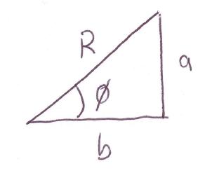
Vector R with sides “a” and “b”
In order to analyze this mechanical system vector loop equations are needed.
A vector shorthand is similar to describing the length R of the triangle into the sides “a” and “b.” Coordinate systems a basically vector systems that describe positions of objects with X and Y componentThe “a” side of the triangle is our “Y” (or up and down) vertical component and the “b”side of the triangle is our “X” (or side to side) horizontal component.
In a vector loop we look at the “X” positions by themselves and we look at the “Y” positions by themselves.
So lets start with the suspension component and evaluate the “X” profile:
X Vector Loop Equation Set
Remember our trig and how it applies to triangles. First in order to evaluate the system we need to break it into three different right triangles. What?! That is right three different triangles like so:
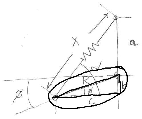
First Triangle Set
The first triangle is Rbc with angle THETA.
Second Triangle (which actually is not a triangle in the techincal sense. It has an angle of zero for its sides)
The second triangle is actually not a right triangle in the formal sense but a triangle with an angle being zero, so it only has one side a. It could easily be transformed into triangle however and be solved in the same manner we are using here however. So for our purposes realize that length a could be moved so it has its own triangle.
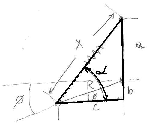
Third Triangle
The third triangle is XC(ba). “b” and “a” form one side of the triangle.
So the X vector loop was solved by going across the bottom section and going back through the top section: like so:
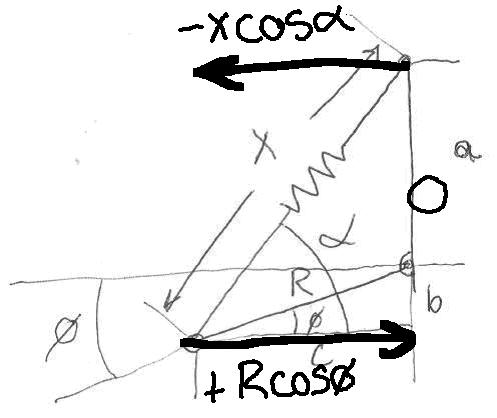
X Loop solution. Go From Left To Right. Adding as you go right and subtracting as you go left.
Proceeding to the right the length “C” is actually RcosTHETA. The next triangle in the “circuit” is a and the length of the side is Zero. We have fully expended any more direction that we can go in the right, so we need to go back to the origin point or to the left and that is +XcosALPHA. Because we are going back, we subtract.
So the general rule is going to the right is positive and any movement to the left is negative or subtracted off.
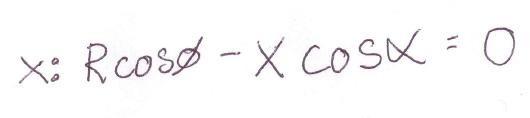
So like we showed before, the vector loop equation for “X” is:
X Vector Loop Equation
The important consideration in all this is the whole system of equations when added together equals zero. (This makes sense, because if you add length C and the suddenly subtract length C you will get Zero. What we have effectively done is described length C with two different triangles that are related to one another.)
Now we need to go to “Y” equations or the “Y” vector loop equation set.
Y Vector Loop Equation
go up and then go down. Positive is up and negative is down:
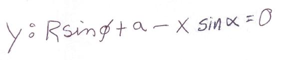
Y Loop Equation Derivation: Proceed UP and then Down to extract the equation. Up is positive and down is negative.
As you can see the first triangle side we encounter is length b which is equivalent to RsinTHETA. The next side is length “a”, so “a” and “b” are added together to make the full height of the triangle. Now that we have gotten as high as the system will let us, we need to go back down. The length down is XsinALPHA.
So this results in the following equation, again all equal to zero.
Y Vector Loop Equation
Now the vector loops are obviously related to eachother, they just describe the X and Y components of the VECTORS or all the moving parts in this system.
The object here is to find out what the length “x” is going to be, since springs are desribed in force by their length or Hooke’s Law: Force Spring = -Kx.
K is the spring rate and “x” is the length. So if K= 100 lb/in then one inch of movement would yield a 100 lb force out of the spring, and a 200 lb force would be equivalent to 2 inches of spring movement.
So our objective is to manipulate the two equations and come out with a solution for “x”. One thing we have in our favor is that we know what Theta is. We know how much the suspension is going to move up and down, we just want to know what “x” is going to be for every degree of THETA.
So what we need to to first is to isolate the x’s into a simple set of equations like so:
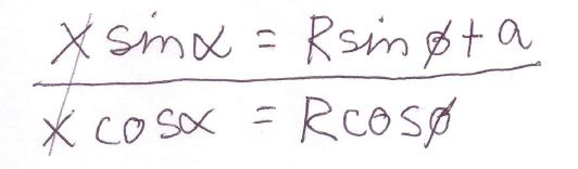
Isolating the “x” and “alpha” unknowns
What we have done is put the Y Loop equation on top of the X loop equation and isolated the unkown sections of the equations to one side. Effectively we have two unknowns. Alpha and “x”. We need to solve for one or the other. But because we are using handy dandy trig, we can easily solve for ALPHA by using the Tangent function like so:
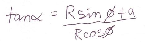
Manipulate the equations which result in Tan(Alpha)
TanALPHA by itself doesn’t help us much, however, if we solve for ALPHA we can then define “x” relative to ALPHA. So we need to solve ALPHA.
How do we do that? Well in Trigonometry there is what is called an inverse-tangent, or an inverse-sine, or an inverse-cosine. Kind of like running the equation backwards, or running tangent backwards.
So an inverse-tangent (or arc-tangent or in computer lingo ATAN) is the solution for ALPHA like so:
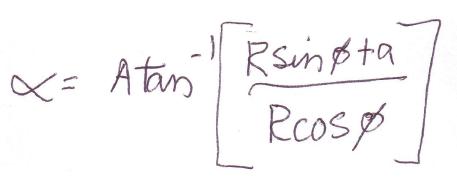
Solving for Alpha using the Inverse Tangent Function (or commonly called Arc Tangent)
If you take a close look at what we just did, we took two sides of the triangle that we know (the vertical and he horizontal components of triangle Xc(ba)) and now are trying to figure out the angle ALPHA.
Tangent ALPHA equals (a+b)/c: or Hieght Over Run
Now that we know what ALPHA is lets solve for “x”:
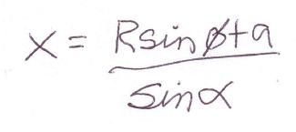
Solving for “x”. “x” is important to use because it is related to the spring length or the amount of force that the spring is putting into the suspension system.
The suspension is now fully described in two dimensional motion. The actually forces that the wheel would see would then be calculated based on this equation set as foundation. The orientation of the wheel, the spring rate and the amount it deflects could all be related by this equation set.
These equations can easily be entered into a spreadsheet. Careful attention however must be taken when dealing with angles however. Angles are typically described in computer language as Radians. Most of us are familiar with Degrees and can readily comprehend what a degree is versus a Radian.
A radian is a form of angular measurement what relates the radius of a circle to the length of the perimeter of the circle. PI radians for example is half a circle or 180 degrees. So a simple conversion is required when using sines, cosines, tangents and so forth, because spreadsheets will use Radians and output radians when used.
Next time we will discuss how to calculate the forces that go into the suspension and what spring rate we should be looking for.